---
title: "JAK inhibitors in PV"
subtitle: "Analysis of the MAJIC-PV Randomized Phase II Trial"
author: "Clinical Research Analysis"
date: today
format:
html:
theme: JOURNAL
toc: true
toc-depth: 3
toc-location: right
number-sections: true
code-fold: true
code-tools: true
fig-width: 9
fig-height: 6
fig-dpi: 300
smooth-scroll: true
highlight-style: github
execute:
echo: true
warning: false
message: false
bibliography: references.bib
---
```{r setup}
#| label: setup
#| include: false
library(tidyverse)
library(gt)
library(survival)
library(survminer)
library(patchwork)
library(scales)
# Define a consistent color palette
pal <- list(
rux = "#C0392B",
bat = "#2980B9",
accent = "#27AE60",
warn = "#F39C12",
dark = "#2C3E50",
light = "#ECF0F1",
cr = "#8E44AD",
no_cr = "#E67E22"
)
# Custom ggplot theme for clinical trial figures
theme_majic <- function(base_size = 13) {
theme_minimal(base_size = base_size) +
theme(
plot.title = element_text(face = "bold", size = rel(1.2), hjust = 0),
plot.subtitle = element_text(color = "grey40", size = rel(0.9), hjust = 0),
plot.caption = element_text(color = "grey50", size = rel(0.7), hjust = 0),
panel.grid.minor = element_blank(),
panel.grid.major = element_line(color = "grey92"),
legend.position = "top",
legend.title = element_text(face = "bold", size = rel(0.85)),
legend.text = element_text(size = rel(0.8)),
axis.title = element_text(face = "bold", size = rel(0.9)),
strip.text = element_text(face = "bold", size = rel(0.9)),
plot.margin = margin(15, 15, 15, 15)
)
}
theme_set(theme_majic())
```
# Study Overview
## Background
Polycythemia vera (PV) is a myeloproliferative neoplasm driven by JAK2 mutations (typically *JAK2*V617F) causing constitutive JAK-STAT signaling and hematopoietic hyperproliferation. Hydroxycarbamide (HC) is the standard first-line cytoreductive therapy, but a subset of patients become **intolerant or resistant** (HC-INT/RES), facing poorer prognosis with limited treatment options.
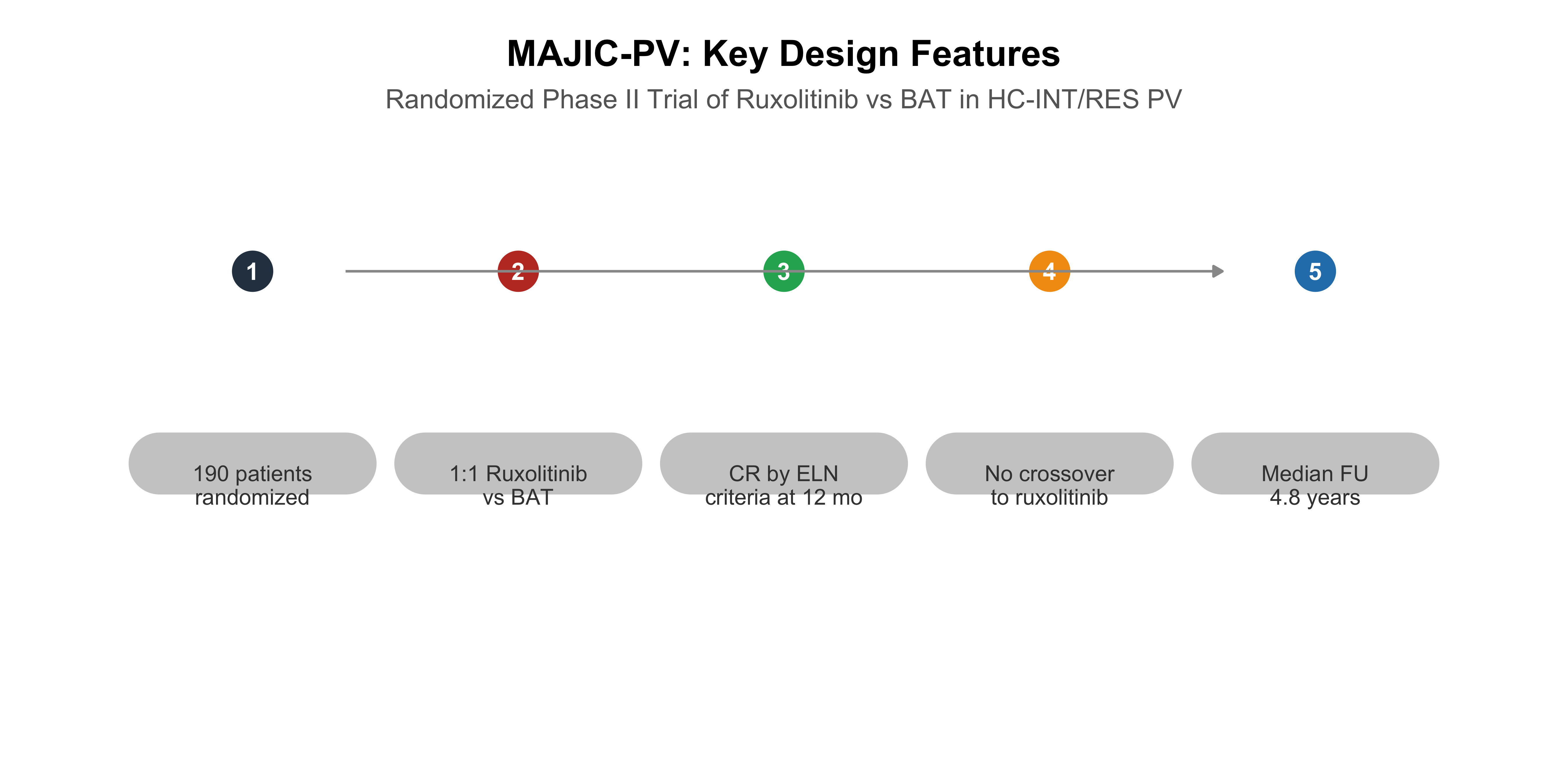
The **MAJIC-PV** trial (ISRCTN61925716) is a randomized, open-label, phase II trial conducted across 38 UK sites evaluating ruxolitinib versus best available therapy (BAT) in HC-INT/RES PV patients. Unlike prior studies (RESPONSE, RESPONSE-2), MAJIC-PV had **no preplanned crossover** and followed patients for up to **60 months**, enabling assessment of long-term clinical and molecular outcomes.
## Trial Design
```{r trial-design-summary}
#| label: fig-trial-design
#| fig-cap: "MAJIC-PV Trial Design Summary"
#| fig-height: 4.5
# Create a visual summary of the trial design
design_data <- tibble(
  phase = factor(
    c("Screening", "Randomization", "Treatment\n& Follow-up", "Primary\nEndpoint", "Long-term\nFollow-up"),
    levels = c("Screening", "Randomization", "Treatment\n& Follow-up", "Primary\nEndpoint", "Long-term\nFollow-up")
  ),
  start = c(0, 1, 2, 3, 4),
  end   = c(1, 2, 3, 4, 5),
  y     = c(0.5, 0.5, 0.5, 0.5, 0.5)
)

key_features <- tibble(
  label = c(
    "190 patients\nrandomized",
    "1:1 Ruxolitinib\nvs BAT",
    "CR by ELN\ncriteria at 12 mo",
    "No crossover\nto ruxolitinib",
    "Median FU\n4.8 years"
  ),
  x = 1:5,
  y = rep(0.5, 5),
  icon_color = c(pal$dark, pal$rux, pal$accent, pal$warn, pal$bat)
)

ggplot(key_features) +
  geom_segment(
    aes(x = x - 0.35, xend = x + 0.35, y = y, yend = y),
    color = "grey80", linewidth = 12, lineend = "round"
  ) +
  geom_point(aes(x = x, y = y + 0.18), size = 8, shape = 21,
             fill = key_features$icon_color, color = "white", stroke = 2) +
  geom_text(aes(x = x, y = y + 0.18), label = 1:5, color = "white",
            fontface = "bold", size = 3.5) +
  geom_text(aes(x = x, y = y - 0.02, label = label), size = 3.2,
            lineheight = 0.9, color = "grey25") +
  geom_segment(
    data = tibble(x = 1.35, xend = 4.65, y = 0.68, yend = 0.68),
    aes(x = x, xend = xend, y = y, yend = yend),
    arrow = arrow(length = unit(0.15, "cm"), type = "closed"),
    color = "grey60", linewidth = 0.5
  ) +
  scale_y_continuous(limits = c(0.25, 0.8)) +
  scale_x_continuous(limits = c(0.4, 5.6)) +
  labs(
    title = "MAJIC-PV: Key Design Features",
    subtitle = "Randomized Phase II Trial of Ruxolitinib vs BAT in HC-INT/RES PV"
  ) +
  theme_void(base_size = 13) +
  theme(
    plot.title    = element_text(face = "bold", hjust = 0.5, size = 15),
    plot.subtitle = element_text(color = "grey40", hjust = 0.5, size = 11),
    plot.margin   = margin(10, 10, 10, 10)
  )
```
# Patient Characteristics
## Baseline Demographics
```{r baseline-table}
#| label: tbl-baseline
#| tbl-cap: "Baseline Patient Characteristics (mITT Population)"
baseline <- tibble(
  Parameter = c(
    "Age, years — median (range)",
    "Sex — Female, n (%)",
    "Sex — Male, n (%)",
    "ECOG 0, n (%)",
    "ECOG 1, n (%)",
    "ECOG 2, n (%)",
    "Disease duration, months — median (range)",
    "Previous lines of therapy — median (range)",
    "HC-Resistant, n (%)",
    "HC-Intolerant, n (%)",
    "Both Resistant & Intolerant, n (%)",
    "History of thrombosis, n (%)",
    "Palpable splenomegaly, n (%)",
    "Hypertension, n (%)",
    "WBC, ×10⁹/L — median (range)",
    "Hemoglobin, g/L — median (range)",
    "Hematocrit — median (range)",
    "Platelets, ×10⁹/L — median (range)",
    "JAK2V617F positive, n (%)"
  ),
  BAT = c(
    "66 (28–85)", "38 (44)", "49 (56)", "59 (68)", "27 (31)", "1 (1)",
    "96 (4–388)", "2 (1–6)", "23 (26)", "37 (43)", "27 (31)",
    "38 (44)", "22 (25)", "25 (29)", "9 (2–37)", "136 (65–163)",
    "0.43 (0.34–0.52)", "356 (99–1,420)", "85 (98)"
  ),
  Ruxolitinib = c(
    "67 (34–88)", "37 (40)", "56 (60)", "57 (61)", "32 (34)", "3 (3)",
    "90 (0–365)", "1 (1–4)", "31 (33)", "43 (46)", "19 (20)",
    "26 (28)", "23 (25)", "33 (35)", "9 (2–73)", "136 (85–173)",
    "0.43 (0.28–0.57)", "401 (61–1,546)", "89 (96)"
  ),
  Overall = c(
    "66 (28–88)", "75 (42)", "105 (58)", "116 (64)", "59 (33)", "4 (2)",
    "91 (0–388)", "1 (1–6)", "54 (30)", "80 (44)", "46 (26)",
    "64 (36)", "45 (25)", "58 (32)", "9 (2–73)", "136 (65–173)",
    "0.43 (0.28–0.57)", "368 (61–1,546)", "174 (97)"
  )
)

baseline |>
  gt() |>
  tab_header(
    title = md("**Baseline Characteristics — MAJIC-PV**"),
    subtitle = md("Modified Intention-to-Treat Population (N = 180)")
  ) |>
  cols_label(
    Parameter   = "",
    BAT         = md("**BAT**<br>(n = 87)"),
    Ruxolitinib = md("**Ruxolitinib**<br>(n = 93)"),
    Overall     = md("**Overall**<br>(N = 180)")
  ) |>
  tab_row_group(label = md("**JAK2 Mutation**"), rows = 19) |>
  tab_row_group(label = md("**Laboratory Values**"), rows = 15:18) |>
  tab_row_group(label = md("**Comorbidities & History**"), rows = 12:14) |>
  tab_row_group(label = md("**HC Status**"), rows = 9:11) |>
  tab_row_group(label = md("**Disease History**"), rows = 7:8) |>
  tab_row_group(label = md("**Performance Status**"), rows = 4:6) |>
  tab_row_group(label = md("**Demographics**"), rows = 1:3) |>
  tab_style(
    style = cell_fill(color = "#F8F9FA"),
    locations = cells_body(rows = seq(1, 19, by = 2))
  ) |>
  tab_style(
    style = cell_text(weight = "bold"),
    locations = cells_row_groups()
  ) |>
  tab_options(
    table.font.size  = px(13),
    heading.title.font.size = px(18),
    heading.subtitle.font.size = px(13),
    column_labels.border.top.width = px(3),
    column_labels.border.top.color = pal$dark,
    column_labels.border.bottom.width = px(2),
    column_labels.border.bottom.color = pal$dark,
    table_body.border.bottom.width = px(2),
    table_body.border.bottom.color = pal$dark,
    row_group.border.top.width = px(1),
    row_group.border.top.color = "grey80"
  ) |>
  tab_source_note(
    source_note = md("*BAT = Best Available Therapy; ECOG = Eastern Cooperative Oncology Group; HC = Hydroxycarbamide*")
  )
```
## Patient Disposition
```{r patient-flow}
#| label: fig-patient-flow
#| fig-cap: "Patient Disposition Through the MAJIC-PV Trial"
#| fig-height: 5
disposition <- tibble(
  timepoint = factor(
    c("Randomized", "mITT", "1 Year\nOn Treatment", "3 Years\nOn Treatment", "5 Years\nOn Treatment", "Data\nSnapshot"),
    levels = c("Randomized", "mITT", "1 Year\nOn Treatment", "3 Years\nOn Treatment", "5 Years\nOn Treatment", "Data\nSnapshot")
  ),
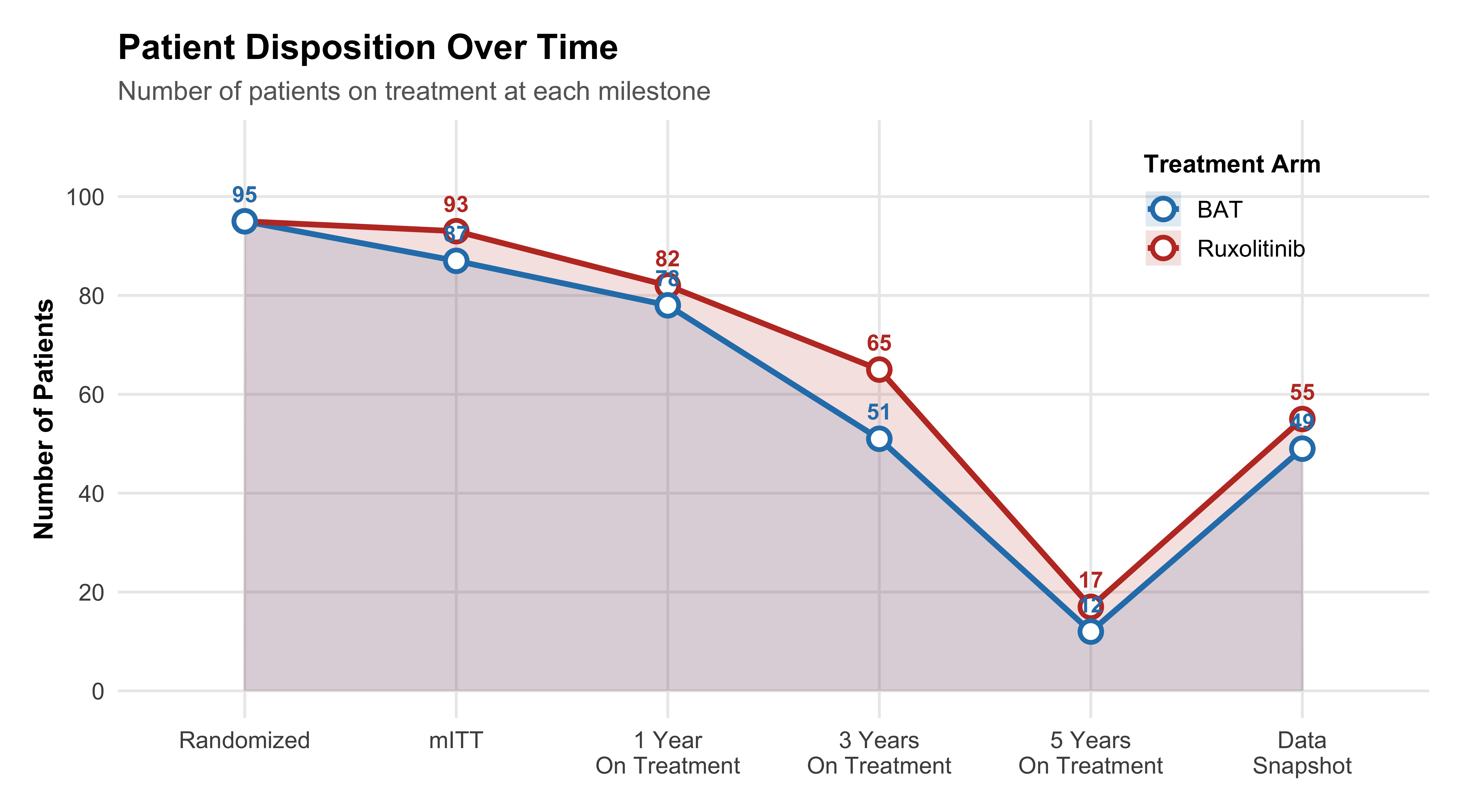
  Ruxolitinib = c(95, 93, 82, 65, 17, 55),
  BAT         = c(95, 87, 78, 51, 12, 49)
) |>
  pivot_longer(cols = c(Ruxolitinib, BAT), names_to = "arm", values_to = "n")

ggplot(disposition, aes(x = timepoint, y = n, fill = arm, group = arm)) +
  geom_area(alpha = 0.15, position = "identity") +
  geom_line(aes(color = arm), linewidth = 1.2) +
  geom_point(aes(color = arm), size = 3.5, shape = 21, fill = "white", stroke = 1.5) +
  geom_text(aes(label = n, color = arm), vjust = -1.2, fontface = "bold", size = 3.5,
            show.legend = FALSE) +
  scale_color_manual(
    values = c("Ruxolitinib" = pal$rux, "BAT" = pal$bat),
    name = "Treatment Arm"
  ) +
  scale_fill_manual(
    values = c("Ruxolitinib" = pal$rux, "BAT" = pal$bat),
    name = "Treatment Arm"
  ) +
  scale_y_continuous(limits = c(0, 110), breaks = seq(0, 100, 20)) +
  labs(
    title    = "Patient Disposition Over Time",
    subtitle = "Number of patients on treatment at each milestone",
    x = NULL, y = "Number of Patients"
  ) +
  theme(legend.position = c(0.85, 0.85))
```
# Efficacy Results
## Primary Endpoint: Complete Response at 12 Months
```{r primary-endpoint}
#| label: fig-primary-endpoint
#| fig-cap: "Primary Endpoint — Complete Response Rate Within 12 Months by ELN Criteria"
#| fig-height: 5.5
cr_data <- tibble(
  arm = factor(c("Ruxolitinib", "BAT"), levels = c("Ruxolitinib", "BAT")),
  cr_rate    = c(43, 26),
  n_respond  = c(40, 23),
  n_total    = c(93, 87),
  pr_rate    = c(54, 67),
  orr        = c(97, 93)
)

# Main CR bar chart
p_cr <- ggplot(cr_data, aes(x = arm, y = cr_rate, fill = arm)) +
  geom_col(width = 0.55, alpha = 0.9, color = "white", linewidth = 0.5) +
  geom_text(aes(label = paste0(cr_rate, "%")),
            vjust = -0.5, size = 6, fontface = "bold", color = "grey20") +
  geom_text(aes(label = paste0("(", n_respond, "/", n_total, ")")),
            vjust = 1.5, size = 3.5, color = "white", fontface = "bold") +
  scale_fill_manual(values = c("Ruxolitinib" = pal$rux, "BAT" = pal$bat)) +
  scale_y_continuous(limits = c(0, 55), labels = label_percent(scale = 1)) +
  annotate("segment", x = 1, xend = 2, y = 48, yend = 48, linewidth = 0.5) +
  annotate("segment", x = 1, xend = 1, y = 46, yend = 48, linewidth = 0.5) +
  annotate("segment", x = 2, xend = 2, y = 46, yend = 48, linewidth = 0.5) +
  annotate("text", x = 1.5, y = 50, label = "OR = 2.12 (90% CI, 1.25–3.60)\nP = .02",
           size = 3.3, fontface = "italic", color = "grey30") +
  labs(
    title    = "Complete Response Rate (Primary Endpoint)",
    subtitle = "ELN Criteria: Hct <45%, Plt ≤400, WBC ≤10, Normal Spleen",
    x = NULL, y = "Complete Response Rate"
  ) +
  guides(fill = "none")

# Response breakdown stacked bar
response_data <- tibble(
  arm = rep(factor(c("Ruxolitinib", "BAT"), levels = c("Ruxolitinib", "BAT")), each = 3),
  response = rep(factor(c("CR", "PR", "No Response"), levels = c("No Response", "PR", "CR")), 2),
  rate = c(43, 54, 3, 26, 67, 7)
)

p_response <- ggplot(response_data, aes(x = arm, y = rate, fill = response)) +
  geom_col(width = 0.55, alpha = 0.85, color = "white", linewidth = 0.3) +
  scale_fill_manual(
    values = c("CR" = pal$accent, "PR" = pal$warn, "No Response" = "grey75"),
    name = "Response"
  ) +
  scale_y_continuous(labels = label_percent(scale = 1)) +
  geom_text(aes(label = ifelse(rate > 5, paste0(rate, "%"), "")),
            position = position_stack(vjust = 0.5), color = "white",
            fontface = "bold", size = 3.5) +
  labs(
    title    = "Overall Response Breakdown",
    subtitle = "CR + PR + No Response",
    x = NULL, y = "Proportion of Patients (%)"
  )

p_cr + p_response +
  plot_annotation(
    title = "MAJIC-PV: Efficacy Outcomes at 12 Months",
    theme = theme(plot.title = element_text(face = "bold", size = 16, hjust = 0.5))
  )
```
## Efficacy Summary Table
```{r efficacy-table}
#| label: tbl-efficacy
#| tbl-cap: "Summary of Key Efficacy Outcomes"
efficacy <- tibble(
  Endpoint = c(
    "Complete Response (CR) at 12 months",
    "Partial Response (PR) at 12 months",
    "Overall Response Rate (CR + PR)",
    "Duration of CR",
    "Event-Free Survival",
    "Thromboembolic Event-Free Survival",
    "Patients with ≥1 Venesection",
    "Total Venesections",
    "TSS Reduction ≥50%"
  ),
  Ruxolitinib = c(
    "43% (40/93)", "54% (50/93)", "97%",
    "HR 0.38", "HR 0.58", "HR 0.56",
    "29% (27/93)", "83", "61% (36/59)"
  ),
  BAT = c(
    "26% (23/87)", "67% (58/87)", "93%",
    "Reference", "Reference", "Reference",
    "52% (45/87)", "307", "30% (17/56)"
  ),
  Effect_Size = c(
    "OR 2.12 (90% CI, 1.25–3.60)",
    "—",
    "—",
    "HR 0.38 (95% CI, 0.24–0.61)",
    "HR 0.58 (95% CI, 0.35–0.94)",
    "HR 0.56 (95% CI, 0.32–1.00)",
    "—",
    "73% fewer venesections",
    "—"
  ),
  P_value = c(
    ".02", "—", "—",
    "<.001", ".03", ".05",
    "—", "—", ".001"
  )
)

efficacy |>
  gt() |>
  tab_header(
    title    = md("**Key Efficacy Outcomes — MAJIC-PV**"),
    subtitle = md("Ruxolitinib vs Best Available Therapy | Median Follow-up: 4.8 Years")
  ) |>
  cols_label(
    Endpoint    = md("**Endpoint**"),
    Ruxolitinib = md("**Ruxolitinib**<br>(n = 93)"),
    BAT         = md("**BAT**<br>(n = 87)"),
    Effect_Size = md("**Effect Size**"),
    P_value     = md("***P* value**")
  ) |>
  tab_style(
    style = list(cell_text(weight = "bold"), cell_fill(color = "#E8F5E9")),
    locations = cells_body(columns = P_value, rows = P_value %in% c(".02", "<.001", ".03", ".05", ".001"))
  ) |>
  tab_style(
    style = cell_fill(color = "#F8F9FA"),
    locations = cells_body(rows = seq(1, 9, by = 2))
  ) |>
  tab_options(
    table.font.size = px(12),
    heading.title.font.size = px(17),
    column_labels.border.top.width = px(3),
    column_labels.border.top.color = pal$dark,
    column_labels.border.bottom.width = px(2),
    column_labels.border.bottom.color = pal$dark,
    table_body.border.bottom.width = px(2),
    table_body.border.bottom.color = pal$dark
  ) |>
  tab_footnote(
    footnote = md("ELN criteria: Hematocrit <45% without venesection for 3 months, platelets ≤400×10⁹/L, WBC ≤10×10⁹/L, normal spleen"),
    locations = cells_body(columns = Endpoint, rows = 1)
  ) |>
  tab_footnote(
    footnote = md("EFS = composite of major thrombosis, major hemorrhage, disease transformation, or death"),
    locations = cells_body(columns = Endpoint, rows = 5)
  ) |>
  tab_source_note(
    source_note = md("*OR = Odds Ratio; HR = Hazard Ratio; TSS = Total Symptom Score*")
  )
```
## Kaplan-Meier Survival Analysis
### Event-Free Survival by Treatment Arm
```{r efs-km}
#| label: fig-efs
#| fig-cap: "Event-Free Survival by Treatment Arm"
#| fig-height: 6
# Reconstruct approximate KM data from published number-at-risk tables
set.seed(42)

# Generate simulated survival data matching published curves
n_rux <- 93; n_bat <- 87

# EFS data matching published HRs and curves
generate_efs <- function(n, rate, censor_rate) {
  event_times  <- rexp(n, rate = rate)
  censor_times <- rexp(n, rate = censor_rate)
  time <- pmin(event_times, censor_times, 5)
  status <- as.numeric(event_times <= censor_times & event_times <= 5)
  tibble(time = time, status = status)
}

rux_efs <- generate_efs(n_rux, rate = 0.10, censor_rate = 0.12) |> mutate(arm = "Ruxolitinib")
bat_efs <- generate_efs(n_bat, rate = 0.18, censor_rate = 0.12) |> mutate(arm = "BAT")
efs_data <- bind_rows(rux_efs, bat_efs) |>
  mutate(arm = factor(arm, levels = c("Ruxolitinib", "BAT")))

fit_efs <- survfit(Surv(time, status) ~ arm, data = efs_data)

# Custom KM plot
efs_plot <- ggsurvplot(
  fit_efs,
  data = efs_data,
  palette      = c(pal$rux, pal$bat),
  risk.table   = TRUE,
  risk.table.col = "strata",
  risk.table.height = 0.25,
  conf.int     = TRUE,
  conf.int.alpha = 0.12,
  pval         = FALSE,
  legend.labs  = c("Ruxolitinib", "BAT"),
  legend.title = "Treatment",
  xlab         = "Time Since Randomization (years)",
  ylab         = "Event-Free Survival (%)",
  break.time.by = 1,
  surv.scale   = "percent",
  ggtheme      = theme_majic(),
  risk.table.y.text = FALSE,
  fontsize     = 3.5
)

# Add annotation for HR
efs_plot$plot <- efs_plot$plot +
  annotate("text", x = 3.5, y = 0.35,
           label = "Published: HR 0.58\n(95% CI, 0.35–0.94)\nP = .03",
           size = 3.5, fontface = "italic", color = "grey30",
           hjust = 0.5) +
  labs(
    title    = "Event-Free Survival (EFS)",
    subtitle = "Composite: major thrombosis, hemorrhage, transformation, or death"
  )

print(efs_plot)
```
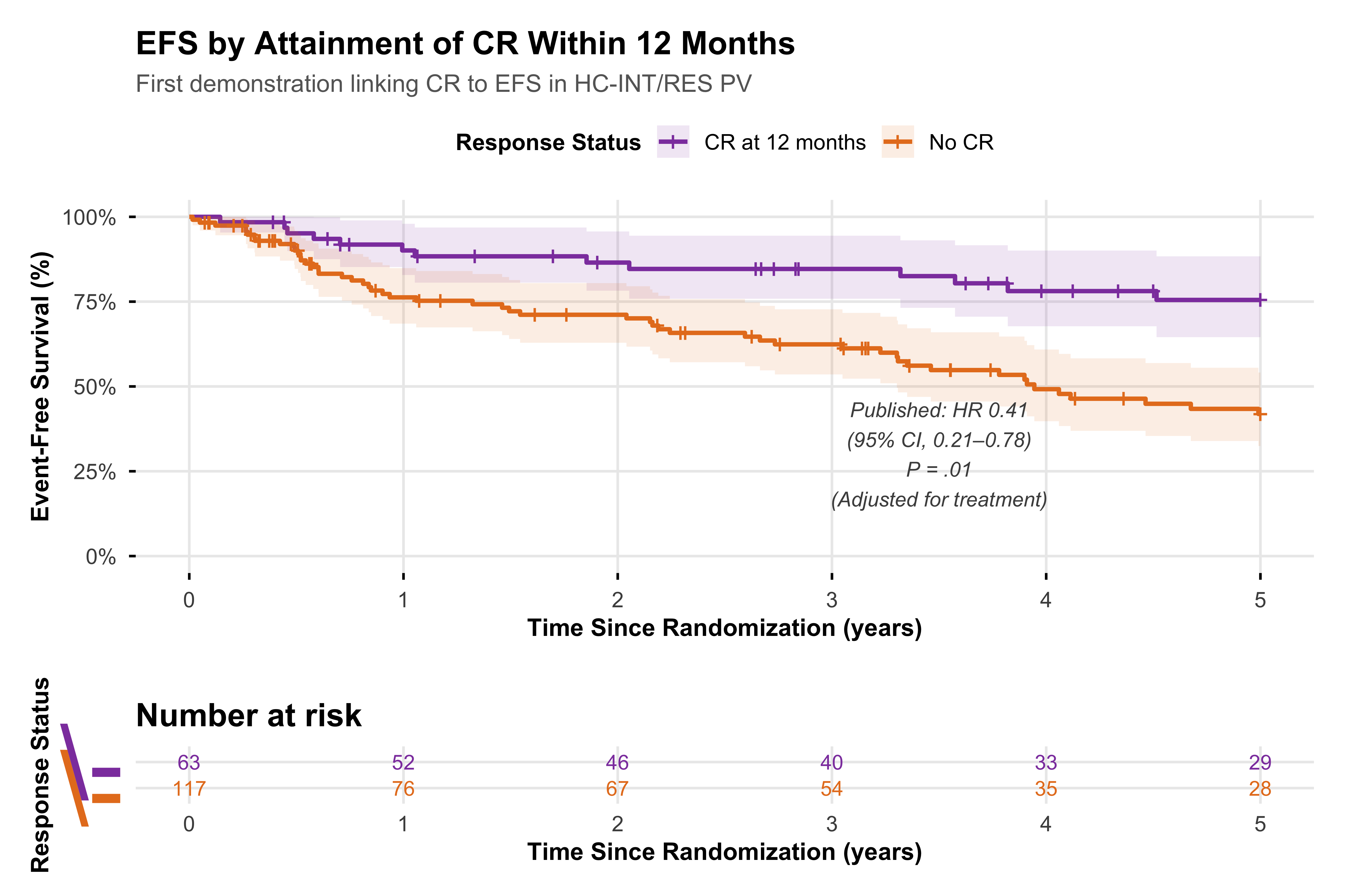
### Event-Free Survival by CR Attainment
```{r efs-cr}
#| label: fig-efs-cr
#| fig-cap: "Event-Free Survival by Attainment of Complete Response Within 12 Months"
#| fig-height: 6
# Generate data matching published CR vs No CR curves
cr_efs <- generate_efs(63, rate = 0.07, censor_rate = 0.10) |> mutate(group = "CR at 12 months")
nocr_efs <- generate_efs(117, rate = 0.16, censor_rate = 0.11) |> mutate(group = "No CR")
cr_data_km <- bind_rows(cr_efs, nocr_efs) |>
  mutate(group = factor(group, levels = c("CR at 12 months", "No CR")))

fit_cr <- survfit(Surv(time, status) ~ group, data = cr_data_km)

cr_plot <- ggsurvplot(
  fit_cr,
  data = cr_data_km,
  palette      = c(pal$cr, pal$no_cr),
  risk.table   = TRUE,
  risk.table.col = "strata",
  risk.table.height = 0.25,
  conf.int     = TRUE,
  conf.int.alpha = 0.12,
  pval         = FALSE,
  legend.labs  = c("CR at 12 months", "No CR"),
  legend.title = "Response Status",
  xlab         = "Time Since Randomization (years)",
  ylab         = "Event-Free Survival (%)",
  break.time.by = 1,
  surv.scale   = "percent",
  ggtheme      = theme_majic(),
  risk.table.y.text = FALSE,
  fontsize     = 3.5
)

cr_plot$plot <- cr_plot$plot +
  annotate("text", x = 3.5, y = 0.30,
           label = "Published: HR 0.41\n(95% CI, 0.21–0.78)\nP = .01\n(Adjusted for treatment)",
           size = 3.5, fontface = "italic", color = "grey30",
           hjust = 0.5) +
  labs(
    title    = "EFS by Attainment of CR Within 12 Months",
    subtitle = "First demonstration linking CR to EFS in HC-INT/RES PV"
  )

print(cr_plot)
```
# Molecular Response
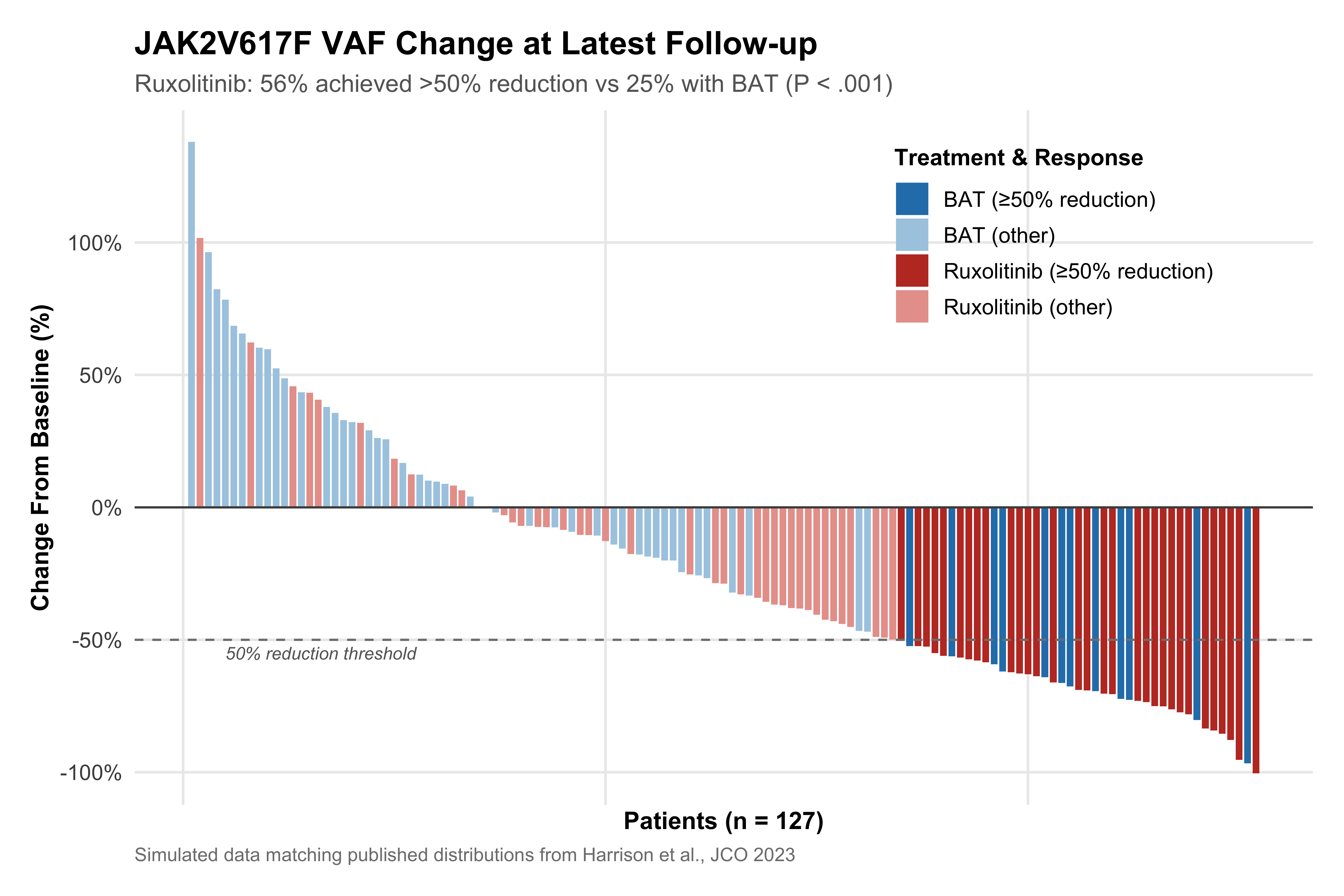
## JAK2V617F Allele Burden Reduction
```{r molecular-waterfall}
#| label: fig-waterfall
#| fig-cap: "Change in JAK2V617F VAF at Latest Time Point vs Baseline"
#| fig-height: 6
set.seed(123)

# Generate waterfall-style data matching published distributions
n_mol_rux <- 70; n_mol_bat <- 57

rux_changes <- c(
  rnorm(39, mean = -65, sd = 18),  # >50% reduction (56%)
  rnorm(11, mean = -35, sd = 8),   # 25-50% reduction
  rnorm(10, mean = -10, sd = 12),  # modest reduction
  rnorm(10, mean = 30, sd = 35)    # increase
)
rux_changes <- sort(rux_changes, decreasing = TRUE)

bat_changes <- c(
  rnorm(14, mean = -62, sd = 15),  # >50% reduction (25%)
  rnorm(8, mean = -30, sd = 10),
  rnorm(15, mean = 5, sd = 20),
  rnorm(20, mean = 55, sd = 45)
)
bat_changes <- sort(bat_changes, decreasing = TRUE)

waterfall <- tibble(
  patient = 1:(n_mol_rux + n_mol_bat),
  change  = c(rux_changes, bat_changes),
  arm     = c(rep("Ruxolitinib", n_mol_rux), rep("BAT", n_mol_bat))
) |>
  arrange(desc(change)) |>
  mutate(
    rank = row_number(),
    fill_color = case_when(
      arm == "Ruxolitinib" & change <= -50 ~ "Ruxolitinib (≥50% reduction)",
      arm == "Ruxolitinib" ~ "Ruxolitinib (other)",
      arm == "BAT" & change <= -50 ~ "BAT (≥50% reduction)",
      TRUE ~ "BAT (other)"
    )
  )

ggplot(waterfall, aes(x = rank, y = change, fill = fill_color)) +
  geom_col(width = 0.8, color = NA) +
  geom_hline(yintercept = 0, linewidth = 0.5, color = "grey30") +
  geom_hline(yintercept = -50, linewidth = 0.5, linetype = "dashed", color = "grey50") +
  annotate("text", x = 5, y = -55, label = "50% reduction threshold",
           size = 3, hjust = 0, color = "grey40", fontface = "italic") +
  scale_fill_manual(
    values = c(
      "Ruxolitinib (≥50% reduction)" = "#C0392B",
      "Ruxolitinib (other)"          = "#E8A09A",
      "BAT (≥50% reduction)"         = "#2980B9",
      "BAT (other)"                  = "#A9CCE3"
    ),
    name = "Treatment & Response"
  ) +
  scale_y_continuous(
    breaks = seq(-100, 200, 50),
    labels = function(x) paste0(x, "%")
  ) +
  labs(
    title    = "JAK2V617F VAF Change at Latest Follow-up",
    subtitle = "Ruxolitinib: 56% achieved >50% reduction vs 25% with BAT (P < .001)",
    x = "Patients (n = 127)", y = "Change From Baseline (%)",
    caption  = "Simulated data matching published distributions from Harrison et al., JCO 2023"
  ) +
  theme(
    axis.text.x  = element_blank(),
    axis.ticks.x = element_blank(),
    legend.position = c(0.78, 0.82)
  )
```
## Molecular Response and Clinical Outcomes
```{r molecular-outcomes}
#| label: tbl-molecular
#| tbl-cap: "Molecular Response at Last Time Point and Key Trial Outcomes"
mol_table <- tibble(
  Outcome = c(
    "Thromboembolic Event", "Hemorrhagic Event",
    "Progression-Free Survival", "Event-Free Survival",
    "Overall Survival", "CR Achieved at 1 Year"
  ),
  All_NR = c("28 (38%)", "23 (31%)", "29 (39%)", "40 (54%)", "18 (24%)", "22 (30%)"),
  All_PR = c("10 (19%)", "5 (9%)", "6 (11%)", "13 (25%)", "4 (8%)", "27 (51%)"),
  All_P  = c(".02", ".004", ".001", ".001", ".01", ".02"),
  RUX_NR = c("10 (32%)", "9 (29%)", "13 (42%)", "16 (52%)", "8 (26%)", "10 (32%)"),
  RUX_PR = c("7 (18%)", "4 (10%)", "3 (8%)", "8 (21%)", "3 (8%)", "22 (56%)"),
  RUX_P  = c(".17", ".04", ".001", ".006", ".04", ".04")
)

mol_table |>
  gt() |>
  tab_header(
    title = md("**Molecular Response & Clinical Outcomes**"),
    subtitle = md("≥50% JAK2 VAF Reduction at Last Time Point")
  ) |>
  tab_spanner(label = md("**All Patients (n = 127)**"), columns = c(All_NR, All_PR, All_P)) |>
  tab_spanner(label = md("**Ruxolitinib (n = 70)**"), columns = c(RUX_NR, RUX_PR, RUX_P)) |>
  cols_label(
    Outcome = md("**Outcome**"),
    All_NR  = md("NR<br>(n = 74)"),
    All_PR  = md("MR<br>(n = 53)"),
    All_P   = md("*P*"),
    RUX_NR  = md("NR<br>(n = 31)"),
    RUX_PR  = md("MR<br>(n = 39)"),
    RUX_P   = md("*P*")
  ) |>
  tab_style(
    style = list(cell_text(weight = "bold"), cell_fill(color = "#E8F5E9")),
    locations = cells_body(
      columns = All_P,
      rows = All_P %in% c(".02", ".004", ".001", ".01")
    )
  ) |>
  tab_style(
    style = list(cell_text(weight = "bold"), cell_fill(color = "#E8F5E9")),
    locations = cells_body(
      columns = RUX_P,
      rows = RUX_P %in% c(".04", ".001", ".006")
    )
  ) |>
  tab_style(
    style = cell_fill(color = "#F8F9FA"),
    locations = cells_body(rows = seq(1, 6, by = 2))
  ) |>
  tab_options(
    table.font.size = px(12),
    heading.title.font.size = px(17),
    column_labels.border.top.width = px(3),
    column_labels.border.top.color = pal$dark,
    column_labels.border.bottom.width = px(2),
    column_labels.border.bottom.color = pal$dark,
    table_body.border.bottom.width = px(2),
    table_body.border.bottom.color = pal$dark
  ) |>
  tab_footnote(
    footnote = "NR = No molecular response (<50% VAF reduction); MR = Molecular response (≥50% VAF reduction)"
  ) |>
  tab_source_note(
    source_note = md("*P values from chi-squared testing. Harrison et al., JCO 2023*")
  )
```
# Genomic Landscape
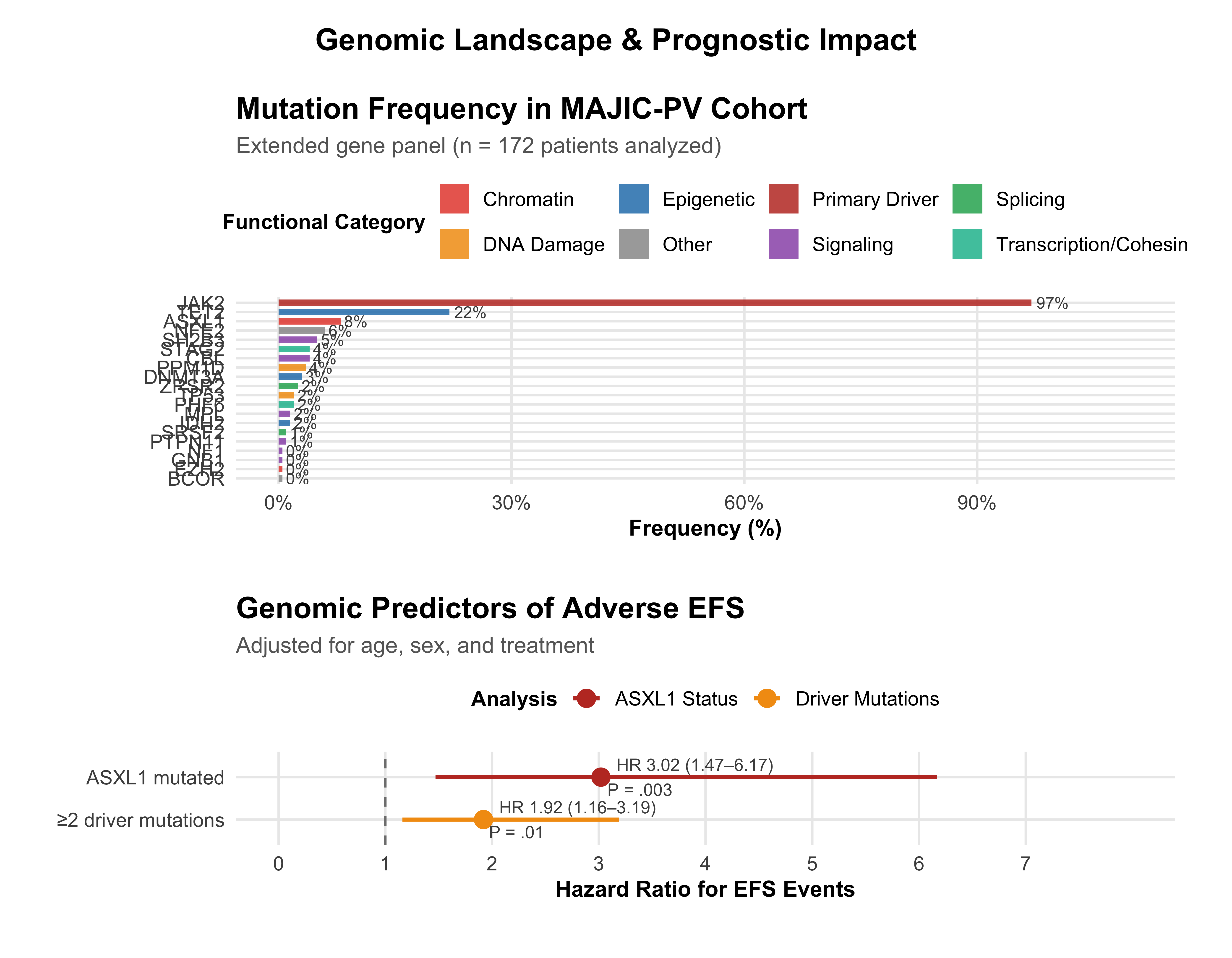
## Mutational Analysis
```{r mutation-landscape}
#| label: fig-mutations
#| fig-cap: "Frequency of Driver Mutations and Impact on Event-Free Survival"
#| fig-height: 7
# Mutation frequency data from the paper
mutations <- tibble(
  gene = c("JAK2", "TET2", "ASXL1", "NFE2", "SH2B3", "CBL", "STAG2",
           "PPM1D", "DNMT3A", "ZRSR2", "TP53", "PHF6", "MPL", "IDH2",
           "SRSF2", "PTPN11", "NF1", "GNB1", "EZH2", "BCOR"),
  frequency = c(97, 22, 8, 6, 5, 4, 4, 3.5, 3, 2.5, 2, 2, 1.5, 1.5, 1, 1, 0.5, 0.5, 0.5, 0.5)
) |>
  mutate(
    gene = fct_reorder(gene, frequency),
    category = case_when(
      gene == "JAK2"                            ~ "Primary Driver",
      gene %in% c("TET2", "DNMT3A", "IDH2")    ~ "Epigenetic",
      gene %in% c("ASXL1", "EZH2")             ~ "Chromatin",
      gene %in% c("SRSF2", "ZRSR2")            ~ "Splicing",
      gene %in% c("TP53", "PPM1D")             ~ "DNA Damage",
      gene %in% c("SH2B3", "CBL", "PTPN11", "NF1", "GNB1", "MPL") ~ "Signaling",
      gene %in% c("STAG2", "PHF6")             ~ "Transcription/Cohesin",
      TRUE                                       ~ "Other"
    )
  )

p_freq <- ggplot(mutations, aes(x = gene, y = frequency, fill = category)) +
  geom_col(width = 0.7, alpha = 0.85) +
  geom_text(aes(label = paste0(round(frequency), "%")),
            hjust = -0.15, size = 3, color = "grey30") +
  coord_flip() +
  scale_fill_manual(
    values = c(
      "Primary Driver"         = pal$rux,
      "Epigenetic"             = pal$bat,
      "Chromatin"              = "#E74C3C",
      "Splicing"               = pal$accent,
      "DNA Damage"             = pal$warn,
      "Signaling"              = "#9B59B6",
      "Transcription/Cohesin"  = "#1ABC9C",
      "Other"                  = "grey60"
    ),
    name = "Functional Category"
  ) +
  scale_y_continuous(limits = c(0, 110), labels = label_percent(scale = 1)) +
  labs(
    title    = "Mutation Frequency in MAJIC-PV Cohort",
    subtitle = "Extended gene panel (n = 172 patients analyzed)",
    x = NULL, y = "Frequency (%)"
  )

# EFS by mutation burden
mutation_efs <- tibble(
  group   = c("Single driver", "≥2 driver mutations"),
  hr      = c(1.00, 1.92),
  hr_low  = c(NA, 1.16),
  hr_high = c(NA, 3.19),
  p_val   = c("Reference", "P = .01")
)

# Also ASXL1-specific
asxl1_efs <- tibble(
  group   = c("ASXL1 wild-type", "ASXL1 mutated"),
  hr      = c(1.00, 3.02),
  hr_low  = c(NA, 1.47),
  hr_high = c(NA, 6.17),
  p_val   = c("Reference", "P = .003")
)

forest_data <- bind_rows(
  mutation_efs |> mutate(analysis = "Driver Mutations"),
  asxl1_efs |> mutate(analysis = "ASXL1 Status")
)

p_forest <- ggplot(forest_data |> filter(!is.na(hr_low)),
                    aes(x = hr, y = group, xmin = hr_low, xmax = hr_high, color = analysis)) +
  geom_vline(xintercept = 1, linetype = "dashed", color = "grey50") +
  geom_pointrange(size = 0.8, linewidth = 1) +
  geom_text(aes(label = paste0("HR ", hr, " (", hr_low, "–", hr_high, ")\n", p_val)),
            hjust = -0.1, size = 3.2, color = "grey30", show.legend = FALSE) +
  scale_color_manual(values = c("Driver Mutations" = pal$warn, "ASXL1 Status" = pal$rux)) +
  scale_x_continuous(limits = c(0, 8), breaks = c(0, 1, 2, 3, 4, 5, 6, 7)) +
  labs(
    title    = "Genomic Predictors of Adverse EFS",
    subtitle = "Adjusted for age, sex, and treatment",
    x = "Hazard Ratio for EFS Events", y = NULL, color = "Analysis"
  )

p_freq / p_forest +
  plot_layout(heights = c(2, 1)) +
  plot_annotation(
    title = "Genomic Landscape & Prognostic Impact",
    theme = theme(plot.title = element_text(face = "bold", size = 16, hjust = 0.5))
  )
```
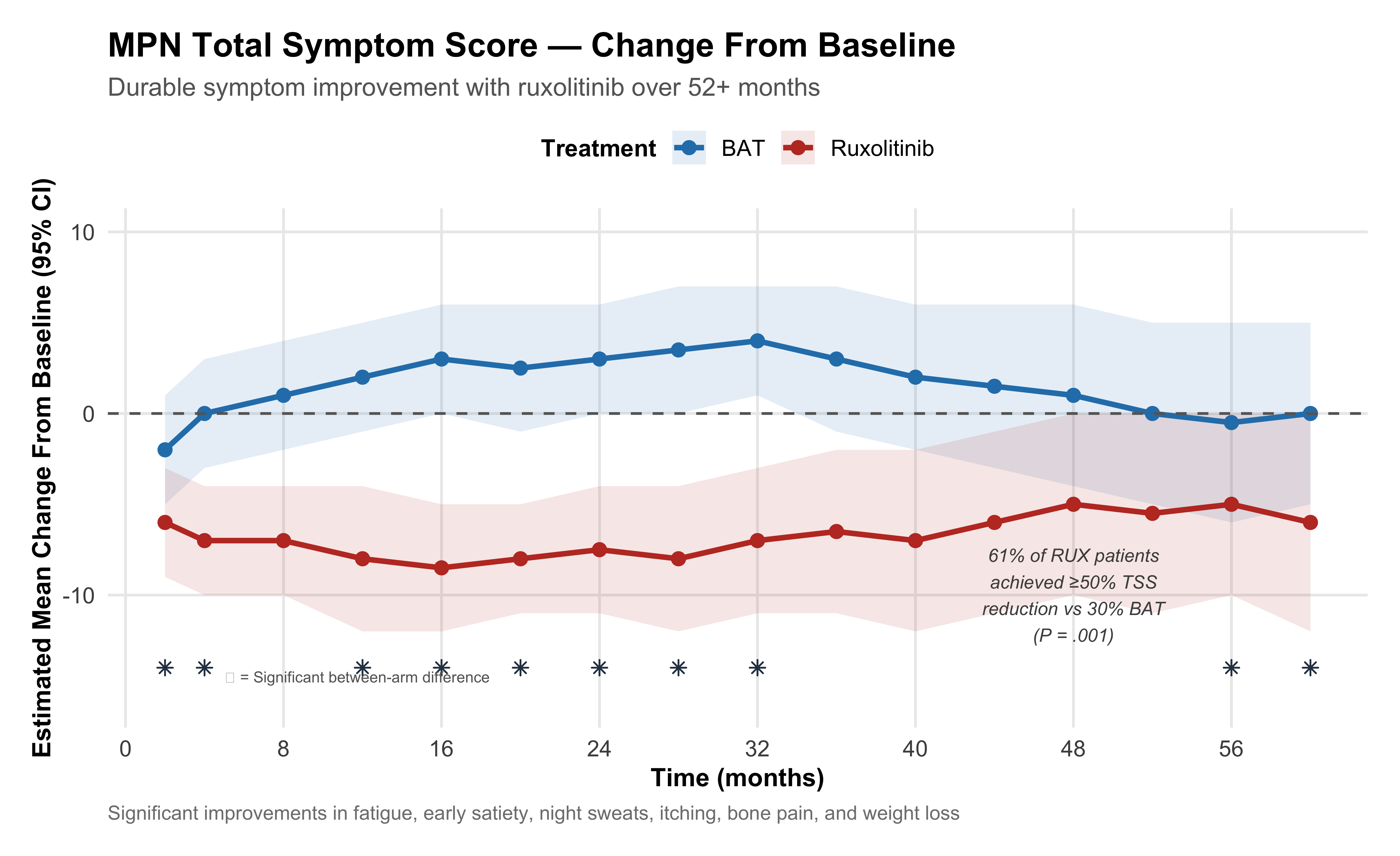
# Symptom Response
```{r symptoms}
#| label: fig-symptoms
#| fig-cap: "MPN Total Symptom Score Change From Baseline Over Time"
#| fig-height: 5.5
# Symptom response data from Figure 4
symptom_data <- tibble(
  month = rep(c(2, 4, 8, 12, 16, 20, 24, 28, 32, 36, 40, 44, 48, 52, 56, 60), 2),
  arm   = rep(c("Ruxolitinib", "BAT"), each = 16),
  mean_change = c(
    # Ruxolitinib: sustained improvement
    -6, -7, -7, -8, -8.5, -8, -7.5, -8, -7, -6.5, -7, -6, -5, -5.5, -5, -6,
    # BAT: worsening then return
    -2, 0, 1, 2, 3, 2.5, 3, 3.5, 4, 3, 2, 1.5, 1, 0, -0.5, 0
  ),
  ci_low = c(
    -9, -10, -10, -12, -12, -11, -11, -12, -11, -11, -12, -11, -10, -11, -10, -12,
    -5, -3, -2, -1, 0, -1, 0, 0, 1, -1, -2, -3, -4, -5, -6, -5
  ),
  ci_high = c(
    -3, -4, -4, -4, -5, -5, -4, -4, -3, -2, -2, -1, 0, 0, 0, 0,
    1, 3, 4, 5, 6, 6, 6, 7, 7, 7, 6, 6, 6, 5, 5, 5
  ),
  n = c(
    55, 56, 53, 48, 43, 46, 45, 37, 44, 42, 43, 38, 32, 26, 21, 22,
    48, 53, 45, 38, 38, 42, 41, 35, 31, 31, 31, 29, 21, 21, 16, 14
  ),
  sig = c(
    TRUE, TRUE, FALSE, TRUE, TRUE, TRUE, TRUE, TRUE, TRUE, FALSE, FALSE, FALSE, FALSE, FALSE, TRUE, TRUE,
    TRUE, TRUE, FALSE, TRUE, TRUE, TRUE, TRUE, TRUE, TRUE, FALSE, FALSE, FALSE, FALSE, FALSE, TRUE, TRUE
  )
)

ggplot(symptom_data, aes(x = month, y = mean_change, color = arm, fill = arm)) +
  geom_ribbon(aes(ymin = ci_low, ymax = ci_high), alpha = 0.12, color = NA) +
  geom_line(linewidth = 1.2) +
  geom_point(size = 2.5) +
  geom_hline(yintercept = 0, linetype = "dashed", color = "grey40") +
  # Mark significant timepoints
  geom_point(
    data = symptom_data |> filter(sig & arm == "Ruxolitinib"),
    aes(x = month, y = -14), shape = 8, size = 2, color = pal$dark, show.legend = FALSE
  ) +
  scale_color_manual(
    values = c("Ruxolitinib" = pal$rux, "BAT" = pal$bat),
    name = "Treatment"
  ) +
  scale_fill_manual(
    values = c("Ruxolitinib" = pal$rux, "BAT" = pal$bat),
    name = "Treatment"
  ) +
  scale_x_continuous(breaks = seq(0, 60, 8)) +
  annotate("text", x = 48, y = -10,
           label = "61% of RUX patients\nachieved ≥50% TSS\nreduction vs 30% BAT\n(P = .001)",
           size = 3, color = "grey30", fontface = "italic") +
  annotate("text", x = 5, y = -14.5,
           label = "✱ = Significant between-arm difference",
           size = 2.5, color = "grey40", hjust = 0) +
  labs(
    title    = "MPN Total Symptom Score — Change From Baseline",
    subtitle = "Durable symptom improvement with ruxolitinib over 52+ months",
    x = "Time (months)", y = "Estimated Mean Change From Baseline (95% CI)",
    caption  = "Significant improvements in fatigue, early satiety, night sweats, itching, bone pain, and weight loss"
  ) +
  coord_cartesian(ylim = c(-16, 10))
```
# Key Findings Summary
```{r summary-forest}
#| label: fig-forest-summary
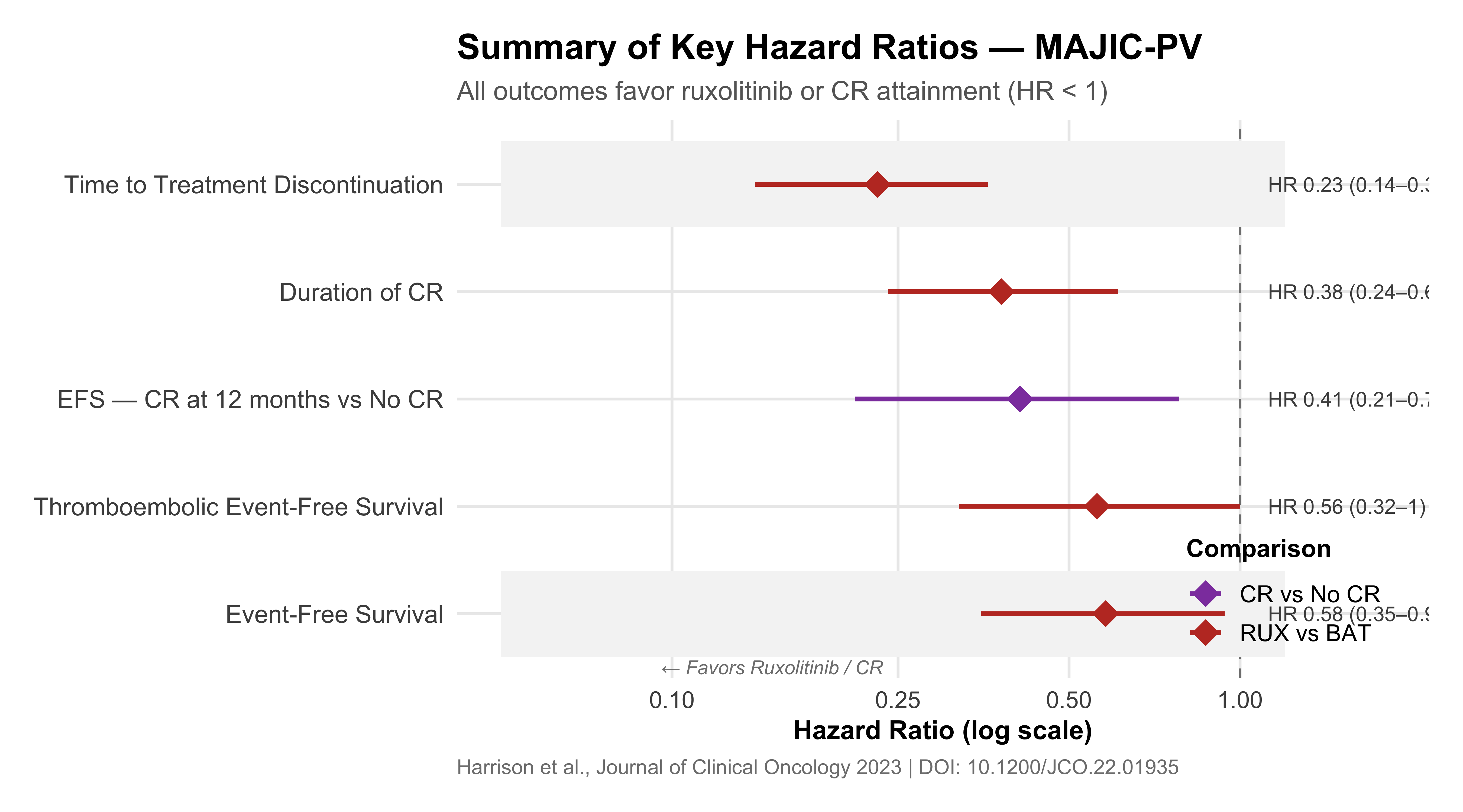
#| fig-cap: "Forest Plot of Key Hazard Ratios Favoring Ruxolitinib"
#| fig-height: 5
forest_summary <- tibble(
  outcome = c(
    "Duration of CR",
    "Time to Treatment Discontinuation",
    "Thromboembolic Event-Free Survival",
    "Event-Free Survival",
    "EFS — CR at 12 months vs No CR"
  ),
  hr      = c(0.38, 0.23, 0.56, 0.58, 0.41),
  ci_low  = c(0.24, 0.14, 0.32, 0.35, 0.21),
  ci_high = c(0.61, 0.36, 1.00, 0.94, 0.78),
  p_value = c("<.001", "<.001", ".05", ".03", ".01"),
  comparison = c("RUX vs BAT", "RUX vs BAT", "RUX vs BAT", "RUX vs BAT", "CR vs No CR")
) |>
  mutate(
    outcome = fct_reorder(outcome, desc(hr)),
    label = paste0("HR ", hr, " (", ci_low, "–", ci_high, ")  P = ", p_value)
  )

ggplot(forest_summary, aes(x = hr, y = outcome)) +
  geom_vline(xintercept = 1, linetype = "dashed", color = "grey50", linewidth = 0.5) +
  geom_rect(
    data = forest_summary |> filter(row_number() %% 2 == 0),
    aes(xmin = 0.05, xmax = 1.2, ymin = as.numeric(outcome) - 0.4, ymax = as.numeric(outcome) + 0.4),
    fill = "grey96", inherit.aes = FALSE
  ) +
  geom_pointrange(
    aes(xmin = ci_low, xmax = ci_high, color = comparison),
    linewidth = 1, size = 1.2, shape = 18
  ) +
  geom_text(aes(label = label, x = 1.12),
            hjust = 0, size = 3.2, color = "grey30") +
  scale_color_manual(
    values = c("RUX vs BAT" = pal$rux, "CR vs No CR" = pal$cr),
    name = "Comparison"
  ) +
  scale_x_continuous(
    limits = c(0.05, 1.8),
    breaks = c(0.1, 0.25, 0.5, 1.0),
    trans  = "log"
  ) +
  labs(
    title    = "Summary of Key Hazard Ratios — MAJIC-PV",
    subtitle = "All outcomes favor ruxolitinib or CR attainment (HR < 1)",
    x = "Hazard Ratio (log scale)", y = NULL,
    caption  = "Harrison et al., Journal of Clinical Oncology 2023 | DOI: 10.1200/JCO.22.01935"
  ) +
  annotate("text", x = 0.15, y = 0.5, label = "← Favors Ruxolitinib / CR",
           size = 3, color = "grey50", fontface = "italic") +
  theme(
    axis.text.y  = element_text(size = 11),
    legend.position = c(0.85, 0.15)
  )
```
# Discussion & Clinical Implications
::: callout-important
## Key Takeaways from MAJIC-PV
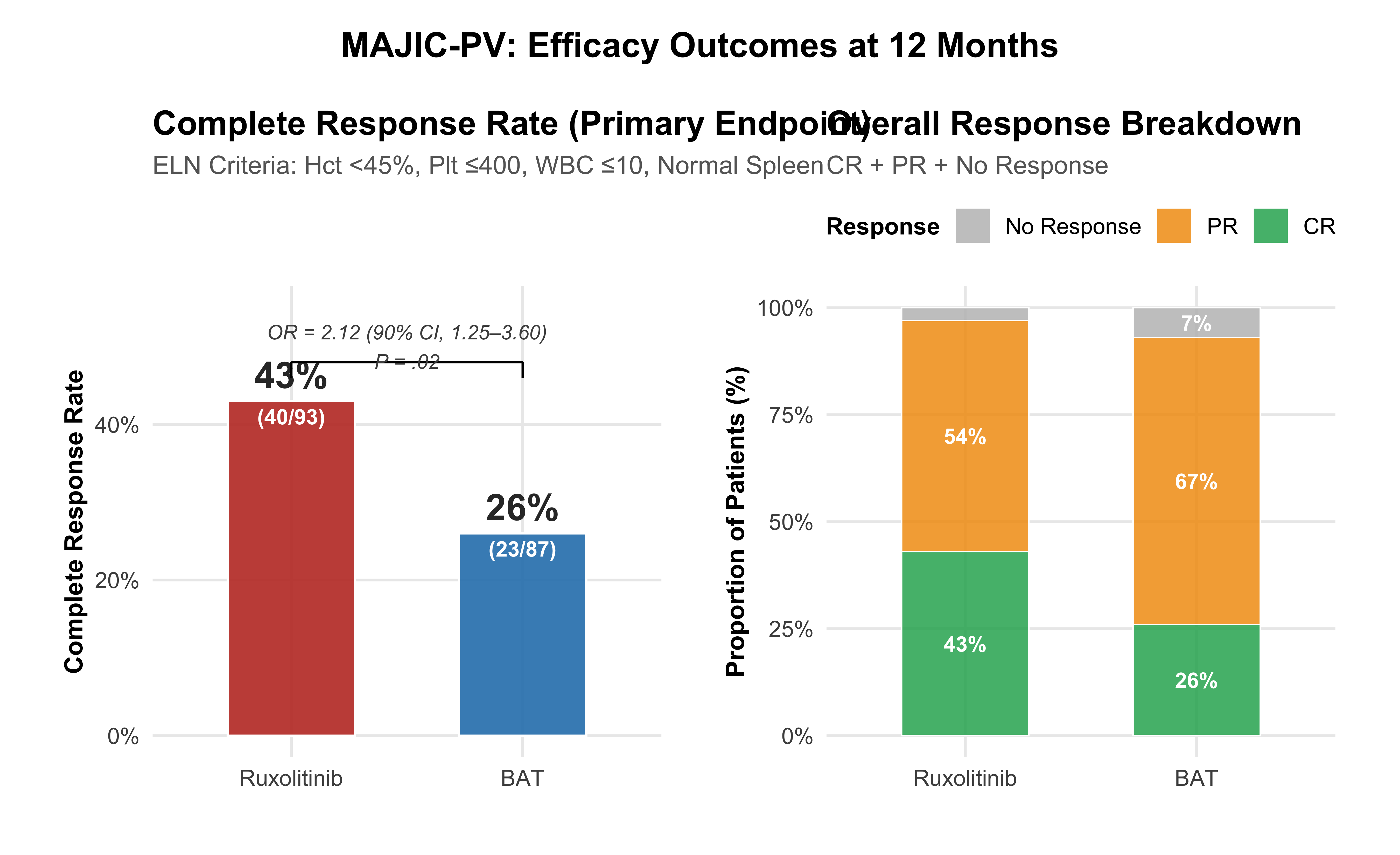
1. **Superior CR rate**: Ruxolitinib achieved 43% CR vs 26% BAT (OR 2.12, P = .02)
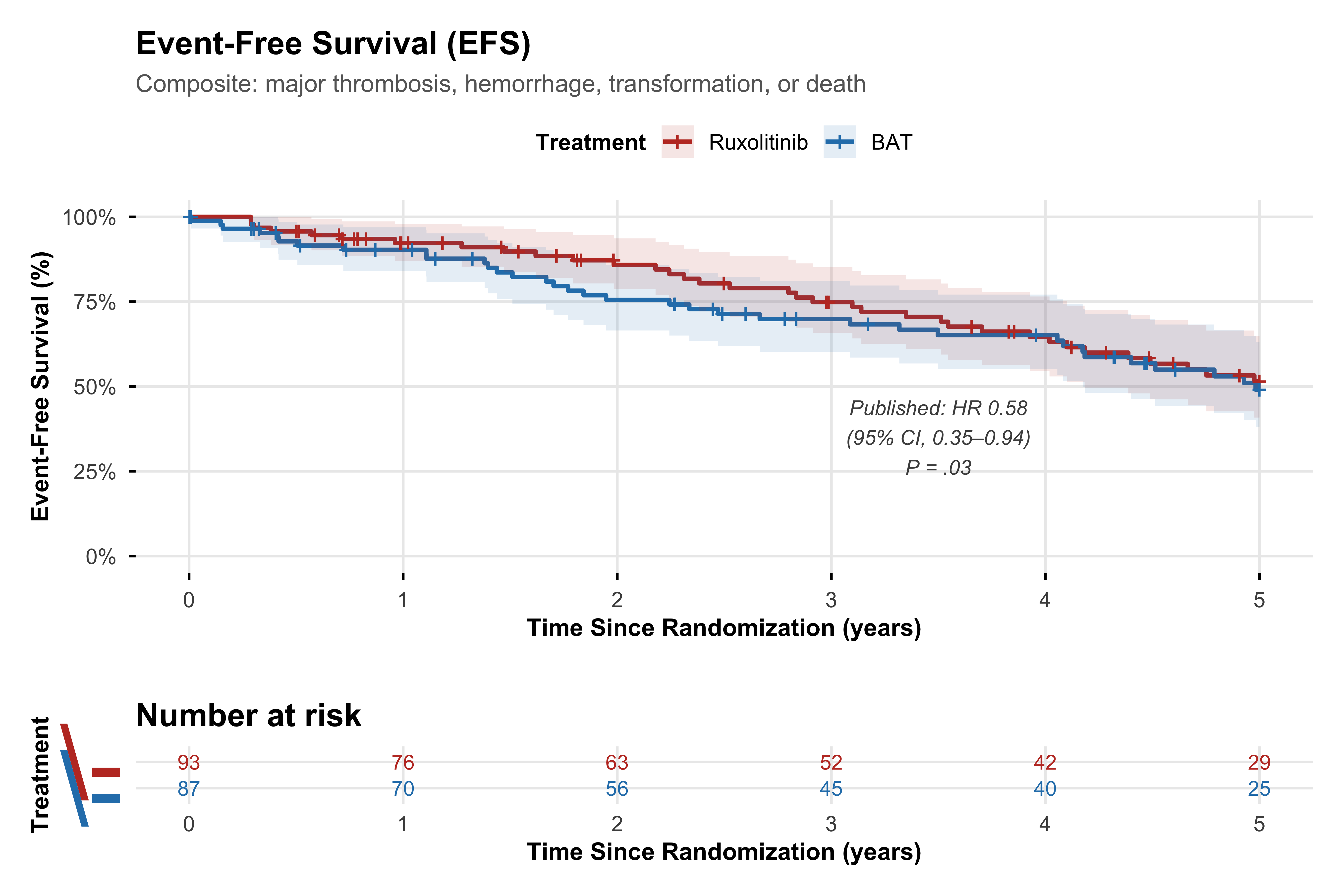
2. **Improved EFS**: First trial to show EFS benefit for ruxolitinib in HC-INT/RES PV (HR 0.58, P = .03)
3. **Molecular response matters**: 50% JAK2V617F VAF reduction linked to improved PFS, EFS, and OS — a novel finding
4. **Durable symptom relief**: 61% of ruxolitinib patients achieved ≥50% TSS reduction, sustained over 52 months
5. **ASXL1 as adverse marker**: ASXL1 mutations conferred 3-fold increased risk of EFS events (HR 3.02, P = .003)
:::
## Comparison with VERIFY Trial (Rusfertide)
While MAJIC-PV established ruxolitinib's benefit in HC-INT/RES PV through JAK inhibition, the emerging VERIFY trial evaluates **rusfertide** (a hepcidin mimetic) as an add-on to current standard of care. These approaches are complementary: ruxolitinib addresses the underlying JAK-STAT pathway activation while rusfertide targets iron-restricted erythropoiesis to control hematocrit independently of cytoreductive mechanisms.
## References
Harrison CN, Nangalia J, Boucher R, et al. Ruxolitinib Versus Best Available Therapy for Polycythemia Vera Intolerant or Resistant to Hydroxycarbamide in a Randomized Trial. *J Clin Oncol*. 2023;41(19):3534-3544. doi:10.1200/JCO.22.01935